#Arch without Pedestal https://pixelfed.social/p/Splines/803615973439041638
#Arch with #Pedestal and Keystone https://pixelfed.social/p/Splines/804537414363507454
#Keystone and #Dentil Details https://pixelfed.social/p/Splines/804548474524642209
#Modillion Details https://pixelfed.social/p/Splines/805587292338863257
#ModernEntablature with Detail https://pixelfed.social/p/Splines/805607059171193759
#Milestone8 - #SimpleIntercolumniation https://pixelfed.social/p/Splines/803106316515798367
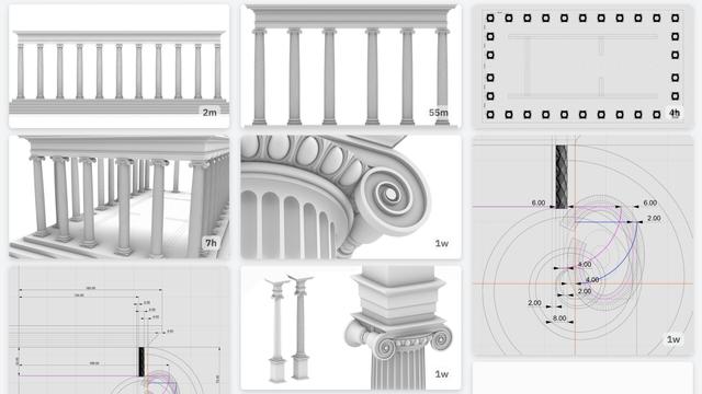
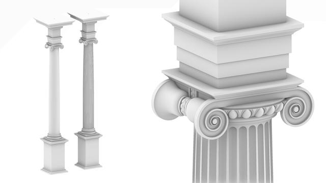
#Milestone7 - Complete #IonicOrder https://pixelfed.social/p/Splines/800050647761776920
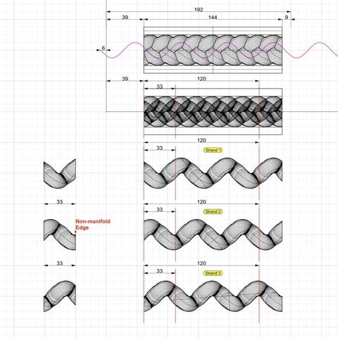
#Milestone6 — #Braids #3StrandBraids https://pixelfed.social/p/Splines/799602946527813102
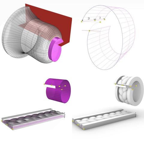
#Milestone5 — #EggsAndDarts https://pixelfed.social/p/Splines/797069447808333887
#Milestone4 — #IonicScroll https://pixelfed.social/p/Splines/795361973789834465
#Milestone3 — #IonicColumn https://pixelfed.social/p/Splines/792803978865652429
#Milestone2 — Classic #IonicEntablature https://pixelfed.social/p/Splines/791021871062069787
#Milestone1 — #IonicPedestal https://pixelfed.social/p/Splines/790752092700055739


Splines (@[email protected])
#Arcade #Intercolumniation without #Pedestal In https://pixelfed.social/p/Splines/803089629244302486, we saw #simpleIntercolumniation, also known as #Architravato. Roman architects combined columns with walls thick enough to bury half of the column width inside the walls and added arches to them for better load distribution. An arcade (multiple arches) can be run in series along a single wall, or in parallel to form a walkway. They can also be combined in both series and parallel configurations, perhaps the most famous of which is the #Colosseum in Rome. In the Colosseum, the outer walls follow an elliptical curve (even though it looks circular from the outside), and it has multiple tiers of arches in series. The interior has arches in concentric passageways in the lower tiers giving it a lattice-like design. Because arches distribute the load from above, they allow for wider intercolumniation. The rules for #ArcadeIntercolumniation differ depending on whether the columns have pedestals or not. Besides the arch itself, which is part of the wall, the figure shows some new architectural elements. The narrow part of the wall immediately behind a column is known as a #pier. The visible face of a pier between a column and the opening under the arch is known as #alette. The base of the pier has a molding, the flat part of which has the same height as the column base (µ) while the rest follows the #fillet and #cavetto or #conge of the #shaft. As we move up the pier, there is a horizontal molding known as #impost just below where the arc of the arch starts. The impost wraps around on the sides of the pier. Around the arc is a circular molding known as #archivolt, the bottom portion of which has a #fascia that is aligned with the face of the wall. The wall itself extends all the way to the top of the #entablature. It is worth noting that the entablature is repeated on the wall. It doesn't end at the columns and has two "outside" corners and one "inside" corner.