New paper, with Kirill Kovalenko, Gonzalo Contreras, Stefano Boccaletti and Rubén Sánchez.
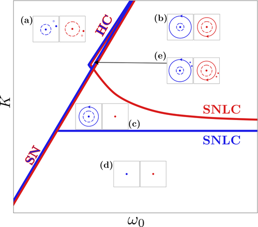
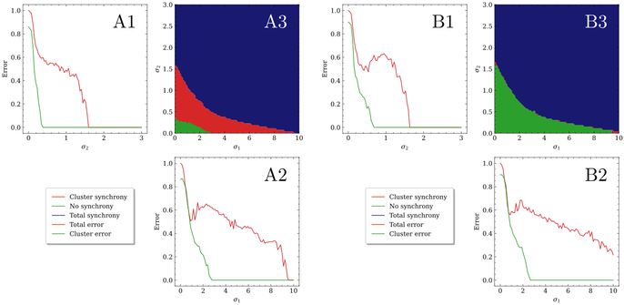
People have noticed that, in higher-order networks, synchronization is often explosive, and that cluster synchronization happens very rarely, if ever. We explain why, by showing that symultaneous dynamical equitability across layers or interaction orders is necessary and sufficient for cluster synchronization, except if the coupling functions depend linearly on each other. Since the probability of randomly satisfying this condition is exceedingly low, cluster synchronization is precluded in such networks.
https://www.nature.com/articles/s42005-026-02543-5
#mathematics #physics #science #networks #complexity #HigherOrderNetworks #MultiplexNetworks #synchronization #dynamicalsystems #graphs #graphtheory #equitability #ClusterSynchronization #ExplosiveSynchronization