Add some swag to your ggplots, with fontawesome symbols and colors: https://nrennie.rbind.io/blog/adding-social-media-icons-ggplot2/ #rstats #ggplot #fontawesome #ggtext
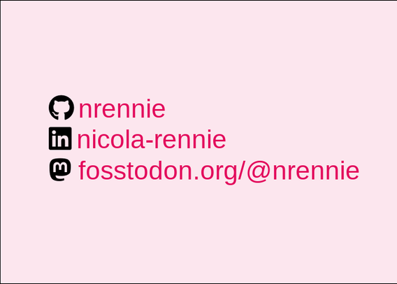
Adding social media icons to charts with {ggplot2} – Nicola Rennie
Adding social media icons to your data visualisation is a great, concise way to put your name on your work, and make it easy for people to find your profile from your work. This blog post explains how to add social media icons to {ggplot2} charts.