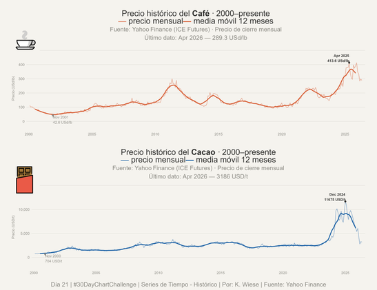
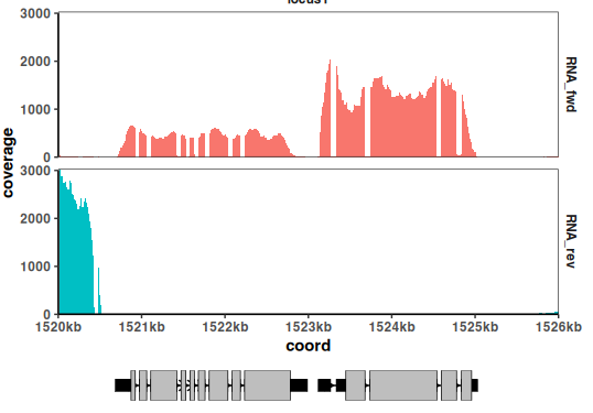
#cowplot is a great package to combine #ggplot2 plots for publications. #patchwork is an alternative that better manages alignment of the plot axes. For example, adding an independent annotation plot (#ggtranscript) to a genome coverage RNA seq plot (#tidyCoverage) can be done with:

coverageplot / annotationplot + plot_layout(nrow=2, heights=c(10,1)

#rstats #visualisation

Day 20 | Timeseries – Urbanization | #30DayChartChallenge. Visualization made with R using #ggplot2, #sf, #dplyr, #scales, #grid, #ggshadow, #extrafont and #cowplot. | Source: Worldometers
Día 11 | Distribuciones – “Stripes” | #30DayChartChallenge. La visualización fue creada usando R basado en los paquetes: #ggplot2, #dplyr, #sf, #lubridate, #ggtext, #showtext, #RcolorBrewer, #rnaturalearth y #cowplot. Fuente: CHIRPS.
Day 10 | Distributions / Multi – Modal | #30DayChartChallenge. Visualization made with R using #ggplot2, #tidyverse, #cowplot, #stars, #raster, #ggspatial and #sf. Data source: Sentinel-2 MSI (2024)
#TidyTuesday Top-10 IMDb TV Series' holiday-season episodes. The Office has the most (6) episodes, the highest-rated and most voted-upon episode!
Code🔗https://tinyurl.com/tidy-hol-episodes
Tools: #rstats #ggplot2 #cowplot by @[email protected]
Data Credits: @R4DSCommunity
Solutions (and Beyond): ggplot2 - Chapter 8

Annotations