#So...
With #TheRightStaff™️ and #EULaw...
#So...
With #TheRightStaff™️ and #EULaw...
“The Not So Puppet Show #003: The Broken Book of Beasties, Book One: A Book by Any Other Cover, Part One” by Thomas Typewriter – a new script
-----------<.thom.>----------- THE NOT SO PUPPET SHOW An asymmetry without apologies Episode #3 “The Broken Book of BeastiesBook I: A Book by Any Other CoverPart 1” By Thomas Typewriter (c) 2026 jason arcand -----------<:type:>----------- FADE IN The Not So Puppet Show’s short title sequence plays. FADE OUTFADE IN THE BROKEN BOOK OF BEASTIES TITLE SEQUENCEThe title “The Broken Book of Beasties” appears far off in the dark screen, written in bright red flowing script. The […]
———–<.thom.>———– THE NOT SO PUPPET SHOW An asymmetry without apologies Episode #3 “The Broken Book of BeastiesBook I: A Book by Any Other Cover…
#So...
#That's #AllFine... #TheInternetIsStillOn
With #TheRightStaff™️ and #EULaw...
And, we're #LongWeekendReady... #BroughtToYou by #Celcius; #PoweredBy #FloofsAndSparkles
AraInfo vincula a Okupacción con prácticas de acoso extrajudicial y relaciones con la ultraderecha en Aragón
📰 Título original: Okupacción: la organización parapolicial que hace negocio del miedo en Aragón
🤖 IA: Es clickbait ⚠️
👥 Usuarios: Es clickbait ⚠️
Ver resumen IA completo https://es.killbait.com/arainfo-vincula-a-okupaccion-con-practicas-de-acoso-extrajudicial-y-relaciones-con-la-ultraderecha-en-aragon.html?utm_source=masto_es&utm_medium=social&utm_campaign=killbait.masto_es
#so...
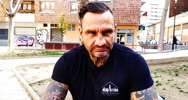
Un reportaje publicado por AraInfo analiza la actividad de Okupacción, una empresa que actúa en Aragón ofreciendo servicios relacionados con desalojos y conflictos de vivienda. El medio describe a la organización como un grupo parapolicial que presuntamente utiliza métodos de presión, intimidación y acoso contra personas vulnerables, especialmente inquilinos con problemas de impago o situaciones de exclusión residencial. Según varios testimonios recogidos en el artículo, miembros de plataformas por la vivienda denuncian amenazas veladas, coacciones y actuaciones fuera de los cauces judiciales habituales. La investigación señala directamente a José Antonio Ramos, gerente de la organización, y destaca sus vínculos políticos con Vox, formación para la que fue candidato municipal en Pinseque. También se mencionan colaboraciones mediáticas y apariciones públicas junto a representantes del partido en Zaragoza. AraInfo sostiene que estas empresas se benefician de un clima de alarma social alimentado por determinados discursos sobre la ocupación de viviendas. El texto también relaciona a Okupacción con intereses inmobiliarios, indicando que Ramos figura como administrador o socio de varias sociedades vinculadas al sector. Además, el artículo compara este tipo de organizaciones con otras empresas similares como Desokupa o Apd Security Iberia. La noticia concluye defendiendo que el fenómeno de la ocupación está sobredimensionado mediáticamente y recuerda que, según datos oficiales citados del Ministerio del Interior, las ocupaciones representan un porcentaje muy reducido del total de viviendas. El reportaje interpreta que el aumento del discurso securitario responde a intereses económicos y políticos ligados al mercado inmobiliario y a sectores de ultraderecha.
#So...
With #TheRightStaff™️ and #EULaw...
#IT's #GoodRhododendronWeather...
And, we're #LongWeekendReady... #BroughtToYou by #Beer; #PoweredBy #FloofsAndSparkles…
Experts Advise Grandparents to Avoid Certain Common Phrases That May Harm Children’s Emotional Well-Being
📰 Original title: It's Time To Stop Saying These 6 Phrases To Your Grandkids. Here's Why.
🤖 IA: It's clickbait ⚠️
👥 Users: It's clickbait ⚠️
#so...
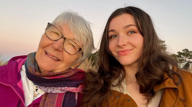
The article explores how well-intentioned comments from grandparents can sometimes negatively affect their grandchildren’s emotional development, self-esteem, and sense of safety. According to pediatric and clinical psychologists, certain common phrases—though often said out of affection or habit—can unintentionally create insecurity, undermine parental authority, or contribute to unhealthy attitudes in children. Experts emphasize that grandparents play an important role in a child’s life, but stress the need for mindful communication. One key concern is encouraging secrecy from parents, such as telling a child not to share certain information, which can weaken trust within the family and potentially expose children to unsafe situations. Another harmful category includes comments about physical appearance or weight, which may contribute to body image issues and long-term self-esteem problems. The article also highlights the risks of commenting on eating habits, such as praising or criticizing how much a child eats, which can interfere with a child’s ability to recognize natural hunger and fullness cues. Additionally, labeling children as “spoiled” or comparing them to others can create feelings of shame or reinforce negative self-perceptions. Experts also warn against pressuring children into physical affection, such as insisting on hugs or kisses, since this may undermine their understanding of personal boundaries and consent. Finally, negative remarks about parents’ decisions or parenting styles should be avoided, as they can place children in the middle of family conflict. Instead, specialists recommend replacing these phrases with open-ended questions, supportive language, and respect for boundaries. The overall message is that small changes in communication can significantly improve emotional safety and strengthen relationships between grandparents and grandchildren.
#So...
With #TheRightStaff™️ and #EULaw...
#DontPanic; #IT's #DefinitelyNotNews...
1: #SpaceKarenX's US$44bn #KiddiePornGeneratingAI #Website is still a #DumpsterFire
2: #Mastodon is #Lovely; and,
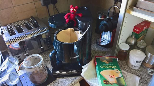
3: #There is a #FreshPotOfCoffee on the #Go...
And, #TheInternetIsStillOn...
#WorkingAsIntended... #StillWorkingAsIntended... #AsIntended
Have #AnotherPrideMonth; #OrSomething...
#RedBeanBear [#CaptainRedBeanBear]... #CaptainRedBeanBearSaysSo...
🧙🛫🤖 🤖🛬🧙 | ☕️️🦹
 🐻🦹☕️
🐻🦹☕️
#ContainsZeroPercentMastodonSocial #AsIntended #TooOldForALTText #MFFS #NoAgeVerificationRequired


#So...
With #TheRightStaff™️ and #EULaw...
Denuncian coordinación policial y amenazas a la comunidad de Errekaleor tras ataque violento
📰 Título original: Vecinas de Errekaleor: “Nos quieren dividir y enfrentar a los de abajo contra los de abajo”
🤖 IA: Es clickbait ⚠️
👥 Usuarios: Es clickbait ⚠️
Ver resumen IA completo: https://es.killbait.com/denuncian-coordinacion-policial-y-amenazas-a-la-comunidad-de-errekaleor-tras-ataque-violento.html?utm_source=mastodon_social&utm_medium=social&utm_campaign=killbait_es.mastodon_social
#so...
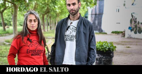
Una vecina de Errekaleor permanece hospitalizada tras sufrir fracturas en el cráneo, mandíbula y un brazo durante un ataque perpetrado por un grupo de personas alojadas en la antigua fábrica de URSSA, armadas con palos y piedras. Miembros del colectivo Errekaleor Auzo Askea denuncian que la Ertzaintza no solo permitió el allanamiento de una vivienda sino que habría facilitado y promovido la agresión, creando un contexto de desgaste político y social en el barrio. Los ataques se enmarcan en una secuencia que incluye la visita del partido Vox, escoltado por la policía, y la difusión de un videorreportaje que enfrenta a okupas nacionales e inmigrantes, según los testimonios. Los vecinos subrayan que estas acciones buscan dividir a la clase trabajadora y debilitar proyectos autogestionados, mientras que el Ayuntamiento y la Consejería de Seguridad califican las acusaciones como inaceptables y acusan al colectivo de clasismo. Aun así, los afectados insisten en que la ocupación responde a la crisis habitacional y que la instrumentalización de personas vulnerables es parte de una estrategia racista y xenófoba. La comunidad mantiene la solidaridad interna y externa, defendiendo la autogestión del barrio y denunciando la connivencia entre fuerzas policiales y discursos de extrema derecha, resaltando la responsabilidad política última del PNV en la gestión de la Ertzaintza.
