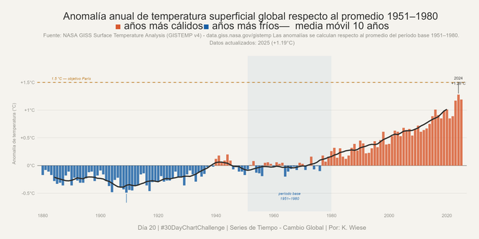
#Día20 | Series de Tiempo – Cambio Global | #30DayChartChallenge | Anomalía anual de temperatura superficial global respecto al promedio 1951–1980. Creada usando #Rstats con #ggplot2, #dplyr, #readr, #scales y #ggtext.

#Day12 | Distributions – FlowingData – ThemeDay | #30DayChartChallenge | Heat Spots in Central America 2020-2024, source: NASA Firms . Built with #RStats using #ggplot2, #dplyr, #readr, #stringr and scales.

#Día4 | Comparaciones – Slope | #30DayChartChallenge. Comportamiento de los focos de calor detectados para los paises de América Central. Creada usando R con #ggplot2, #dplyr, #scales, #readr, #stringr y #ggtext.

#Día3 | Comparación– Mosaico | #30DayChartChallenge. Focos de calor detectados para los paises de América Central. Un gráfico con valores absolutos y otro con valores relativos. Creada usando R con #ggplot2, #treemapify, #dplyr, #scales, #readr y #stringr.

I just learned that #rstats #readr write_csv() returns the data invisibly so you can just insert them within a pipe for a snapshot-then-plot functionality... I always imported magrittr %T>% before but it seems I don't need to use it at all for most cases.